Quantum computing is evolving rapidly across the globe, and Europe is no exception, with significant investments powering new research frontiers. However, a key challenge lies in efficiently orchestrating complex computations that often require integrating classical HPC resources with diverse quantum hardware. In this article we give an overview of ColonyOS, an open-source meta-operating system designed to address this need. We orchestrate distributed computing workflows across heterogeneous environments, including cloud, HPC, standalone workstations, and can be extended towards quantum systems.

The following sections discuss the benefits of such orchestration, highlight key ColonyOS features, and showcase example applications in managing quantum computations. ColonyOS has the potential to streamline hybrid calculations and accelerate the path towards quantum-accelerated supercomputing.

The need for distributed quantum computing

Quantum computing scientists and engineers across different disciplines need to leverage classical and quantum resources in their workflows. They need to develop and test algorithms locally on their personal computers before scaling them up to more complex environments. This iterative process involves expanding the algorithm in terms of parameters, noise models, system complexity, and other details. The next step is to run the workflow on a quantum computer with a few qubits.

Of course, due to the limited accessibility to quantum hardware or the limited qubits available, a common target of that workflow is to run it on a powerful computer, which can be an HPC resource capable of simulating hundreds of qubits with the help of some packages and software development kits. Such solutions have the potential to use extensive resources, making it suitable to distribute the workflow over multiple compute resources. For reusability, users require the ability to access those resources seamlessly, saving time by storing profiles of the hardware that this specific workflow can run on across different European compute infrastructures.

Leveraging ColonyOS for distributed quantum computing

ColonyOS is an open-source meta-operating system designed to streamline workload execution across diverse and distributed computing environments. This includes cloud, edge, HPC, and IoT. More details are provided in the arXiv article. This capability makes it well-suited for managing complex, resource-intensive quantum computing tasks. The software is available under the MIT Licence and you can access it on GitHub. Comprehensive tutorial notebooks are also available to facilitate onboarding.

Key features of ColonyOS that would help drive quantum-accelerated supercomputing

ColonyOS offers several key features that could enable managing the quantum computing workflows and advancing quantum-accelerated supercomputing.

Distributed microservice architectures

ColonyOS employs a microservices architecture, where independent executors handle specific tasks. This design supports distributed quantum computing by allowing quantum tasks to be executed across geographically dispersed quantum and classical computing resources in a hybrid fashion. Executors can be deployed independently and scaled horizontally, ensuring efficient parallel processing.

Workflow orchestration

The platform enables users to define complex, multi-step workflows across distributed executors. This is particularly beneficial for quantum computing applications, which often require iterative execution of quantum circuits, optimisation steps (e.g., variational quantum eigensolver (VQE) algorithms), and hybrid quantum-classical computations. ColonyOS manages dependencies and execution sequencing, ensuring seamless operation across diverse computational systems.

Scalability

Given the potential for node failures in distributed infrastructures, ColonyOS is designed to reassign tasks dynamically if an executor fails. This approach minimises computation disruptions and enhances overall system reliability.

Platform-Agnostic integration

ColonyOS can operate across multiple platforms, including cloud services and HPC environments. This flexibility aligns with the hybrid quantum-classical infrastructures often required for quantum computing workflows, allowing for efficient orchestration of tasks on both classical supercomputers and quantum processors.

The distributed architecture, task orchestration capabilities, and scalability of ColonyOS make it a powerful solution for managing quantum computing workflows. By leveraging ColonyOS, users can efficiently coordinate tasks across quantum and classical computing environments. Thus, accelerating the development and deployment of quantum algorithms that are advancing toward further use in quantum-accelerated supercomputing.

Example: orchestrating and visualising quantum computing workflows with ColonyOS

The following snippets are related to an example where ColonyOS orchestrated Qiskit variational calculations with different noise models. ColonyOS generated multiple simulations accounting for different noise models. For more implementation details and related code, please visit the blog post here.

ColonyOS serialises Qiskit objects, metrics, and metadata from each part of the workflow into an SQLite database. This database is then exposed to localhost via a simple Flask API, which connects to a React frontend that presents two key views of the results data. Both views display the same data and allow ranking across a set of metrics but do so in different ways:

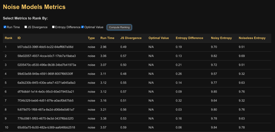
The first way is through the metrics table—a simple (in-development) table that displays each noise simulation computation along with data from its related variational simulation, as shown in the following figure:

The second way is through a workflow graph showing how each step in the workflow is connected and which steps depend on its information, as shown in the following figure:

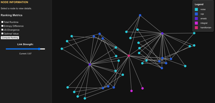
Here, the legend explains which part of the calculation workflow the nodes correspond to. A node information panel displays metrics of the selected node. It allows to compute rankings across nodes (similar to the metrics table shown above in Figure 1) while rescaling and labelling nodes as a function of rank, as depicted here:

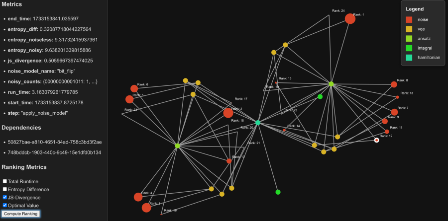
Workth-mentioning that with more complex systems and calculations, the database could present a denser graph providing easily searchable sets of data.

These examples highlight ongoing efforts to integrate ColonyOS into quantum computing workflows—a promising step toward distributed computing orchestration. This work also leveraged graph data analytics to view and analyse quantum computation outcomes. ColonyOS, as part of the European Compute Continuum Initiative, could become a vital part at the orchestration layer for the EuroHPC-JU hybrid quantum-classical infrastructure, enabling seamless utilisation of resources like LUMI-Q and MareNostrum Q with the existing HPC classical resources. To explore ColonyOS further, check out the GitHub repository and the available tutorials.

Acknowledgement

This blog post is based on work by Erik Källman, first presented at the Nordic Quantum Autumn School 2024 and further elaborated in an accompanying blog post here. You can find the original content in Erik Källman’s blog. We adapted and expanded the concepts and implementations with permission to showcase the potential of ColonyOS in distributed quantum computing workflows. We thank Erik Källman for his work in this area and for sharing his insights during the Nordic Quantum Autumn School 2024.

Check our lessons on quantum computing and HPC

At ENCCS we make sure that users get the most out of high performance computing as well as quantum computing. Check our lessons at here.