
This article is the continuation of the first part of “Quantum Computing for Beginners” by Martin N. P. Nilsson, which you can find below. Find the original Arxiv article here. All code examples in this series of tutorials is licensed under the MIT license.
The tutorial was inspired by the “Quantum Autumn School” held in October 2023 and organised by ENCCS, Wallenberg Centre of Quantum Technologies (WACQT), and Nordic-Estonian Quantum Computing e-Infrastructure Quest (NordIQuEst). You can find the full recordings and training material of the Quantum Autumn School below.
Grover’s search is a neat and relatively simple example of how we can use a quantum computer with enough qubits to speed up a calculation. It also shows that one requires quite sophisticated techniques even to solve relatively simple problems with a quantum computer.
Suppose we’ve implemented a function f(x) with quantum gates, where x is represented by N qubits. Let’s also assume that there’s exactly one x_0 such that f(x0) = 1 and f(x) = 0 for all x = x_0. Then, we can use Grover’s search to find x_0 in time O(2^{N/2}), while a naive search would require time O(2^N ), thus a quadratic speedup.
Subroutines
First, let’s look at a function that returns 1 if all qubits are zero, and 0 otherwise:
def zero_booleanOracle(qubits,result): # all qubits zero?
    # if all qubits==0 return 1 else return 0
    for qubit in qubits:             # negate all inputs
        applyGate(X_gate,qubit)
    TOFFn_gate(qubits,result)        # compute AND
    for qubit in qubits:             # restore inputs
applyGate(X_gate,qubit)It simply inverts the qubits with X gates, and then performs an AND using the generalized Toffoli gate. The result is delivered through the ancilla qubit result. Afterward, the input qubits are reset. Such a function is called a Boolean oracle.
For Grover’s algorithm, we use a variant of the above procedure that doesn’t have a result qubit but ‘returns’ the value 1 through a sign change in the contents of the corresponding small cubes. Physicists call this sign change a ‘phase change.’ When returning the value 0, no sign change is made. Such a function is called a phase oracle. A trick to achieve the sign change is to apply Hadamard gates to the controlled bit before and after the Toffoli gate. Which bit is controlled doesn’t matter. Such a gate is exactly the same as a controlled Z gate, so we can write
def zero_phaseOracle(qubits):            # all qubits zero?
    # if all qubits==0 return -weight else return weight
    for qubit in qubits:                 # negate all inputs
        applyGate(X_gate,qubit)
    applyGate(Z_gate,*namestack)         # controlled Z gate
    for qubit in qubits:                 # restore inputs
applyGate(X_gate,qubit)Note that beccause of the symmetry of the controlled Z gate, any order of the qubits is OK. Apply- ing it in the namestack order has the advantage that the qubits don’t need to be moved around.
Finally, we come to our ‘Black box’ function. We also need to express this as a phase oracle, that is, it should give a sign change for the solutions to the function. As an example, right here, we use the function
f(x) =
\begin{cases}
       \text{1} &\quad\text{if all qubits except qubit 1 are one,}\\
       \text{0} &\quad\text{otherwise}
\end{cases}
The implementation is similar to what we did for zero_phaseOracle, but here we only negate qubit 1. Given six qubits, the procedure should negate the weights if the input is 111101 in binary (a programmer might think of this number as -3), otherwise, leave the weights unchanged.
def sample_phaseOracle(qubits):          # sample function
        # if all f(x)==1 return -weight else return weight
    applyGate(X_gate,qubits[1])          # negate qubit 1
    applyGate(Z_gate,*namestack)         # controlled Z gate
applyGate(X_gate,qubits[1]) # restore qubit 1If we wanted to check for -7, we could add one line for negating qubit 3 by applygate(X_gate,qubits[3]) before the application of the Z-gate, and another line for restoring it after the Z-gate. The sample function would then recognize binary 110101.
The Main Loop
Now we’re ready to implement the main loop of Grover’s search. It alternates between running sample_phaseOracle and zero_phaseOracle, applying Hadamard gates between them. It’s really not obvious why this works, but a brief explanation is in the next section. With each iteration, the probabilities of the qubits being ‘right’ gradually improve. So the weight for the small cube that is the solution increases with each iteration. This is called amplitude amplification.
def groverSearch(n, printProb=True):
    optimalTurns = int(np.pi/4*np.sqrt(2**n)-1/2)   # iterations
    qubits = list(range(n))                         # generate qubit names
    for qubit in qubits:                            # initialize qubits
        pushQubit(qubit,[1,1])
    for k in range(optimalTurns):                   # Grover iterations:
        sample_phaseOracle(qubits)                  # apply phase oracle
        for qubit in qubits:                        # H-gate all qubits
            applyGate(H_gate,qubit)
        zero_phaseOracle(qubits)                    # apply 0 phase oracle
        for qubit in qubits:                        # H-gate all qubits
            applyGate(H_gate,qubit)
        if printProb:                               # peek probabilities
            print(probQubit(qubits[0]))             # to show convergence
    for qubit in reversed(qubits):                  # print result
print(measureQubit(qubit),end="")To illustrate the convergence, we print out the bit probabilities for qubit 0 in each iteration. Here’s what a run looks like:
workspace = np.array([[1.]])              # initialize workspace
groverSearch(6) # (only reals used here)[0.43945313 0.56054687]
[0.33325958 0.66674042]
[0.20755294 0.79244706]
[0.09326882 0.90673118]
[0.01853182 0.98146818]
111101It’s clear that the probability of a zero approaches zero and for a one approaches one, so a correct result is likely, but still not entirely certain. One must test it and redo the search if the result turns out to be wrong. Grover’s search doesn’t offer an exponential speedup but ‘only’ a quadratic one. However, one can show that this is the best that we can achieve with a quantum computer.
Once again, it’s clear that the main problem is not calculating the function, as this is done in one sweep for all conceivable arguments by sample_phaseOracle, but in extracting the solution after the calculation.
Why Grover’s Search Works
Let’s see the workspace as a row vector of M = 2^N small cubes again. The sought solution x0 to f(x) = 1 can be described with a ‘one-hot’ encoding as an M-dimensional unit vector
x_0 =(0,0,...,1,...,0),
where only one coordinate (= small cube weight) differs from zero. Let the vector y be another M-dimensional unit vector with a zero where x_0 has a one, while the other coordinates are 1/\sqrt{M-1} so that
y=\frac{1}{\sqrt{M-1}}(1, 1, ..., 0, ..., 1)This vector represents all the small cubes that are not solutions. Since the scalar product x · y = 0, the vectors x and y must be orthogonal. We introduce the vector
z=\frac{1}{\sqrt{M}}(1, 1, ..., 1, ..., 1)= \frac{1}{M}x + \frac{\sqrt{M-1}}{M}ywhich is a linear combination of x and y.
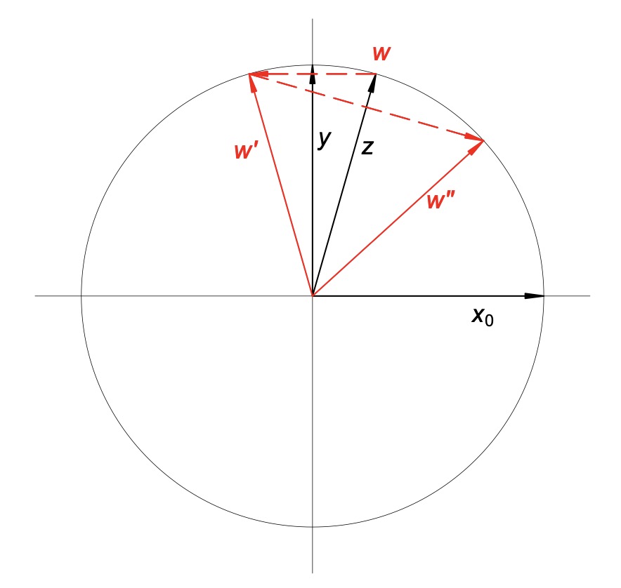
We let the vector w represent the approximation to the solution during Grover’s search and initialize it to z. The first call to the phase oracle sample_phaseOracle reflects w across the y-axis (Fig. 3), to become w′. It’s relatively straightforward to show that the second call, along with the Hadamard gates, then reflects w′ in z, resulting in w′′. This vector is closer to x_0 than w, so we replace w with w′′ and repeat the procedure. It can be calculated that the probability of hitting x_0 is highest after
k=\Bigl\lfloor \frac{\pi}{4}\sqrt{M}-\frac{1}{2}\Bigr\rflooriterations. See references below for details.
- Aaronson, S.: Introduction to Quantum Information Science. Lecture notes. 2018. https://www.scottaaronson.com/qclec.pdf (accessed 2023-11-19)
- Azure Quantum documentation. Microsoft, Inc.
https://learn.microsoft.com/ en-us/azure/quantum/ (accessed 2023-11-19)