
Analysis of traffic flow at E4S (southbound) using deep learning (DL) methods is the subject of an ongoing collaboration between TV, KTH, and ENCCS. The project consists of two parts: 1) modeling flow and link speed at specific links for testing purposes 2) expanding part one to the entire E4S considering correlations between lanes/links.
The answer to why deep learning is considered here for modeling the time series data, here traffic flow, encompasses the different aspects of the problem. First, the chronological order of time-series data makes the modeling a challenging task. Second, DLs are significantly capable of capturing relationships beyond typical linear classical statistical-based models. Third, their capacity of “getting shaped” directly by data without prior assumptions makes them superior to the classical models. For instance, stationary and ergodicity assumptions, which are often not satisfied in data and are crucial for classical models, do not hinder the capability of DL models [1].
Recurrent neural networks are commonly used for time series analysis because they retain ‘memories.’ Classical architectures for sequence-to-sequence modeling are Long short-term memory (LSTM) networks. In part one, LSTM is proposed to study the specific links for testing purposes. Nonetheless, gated recurrent units (GRU) networks, convolutional neural networks (CNN), and temporal neural networks (TCN) were also considered here. CNNs are extremely powerful neural networks (NNs) that have been proven to be very successful in image analysis/classification. The main reason convolutional networks can be successfully applied to the time series data is their unique capability to capture translation invariance features in highly complex data such as images. While CNNs can capture different features of the data, the causal connection is missing. TCN are derivatives of CNNs where the causal convolution enables the network to capture causal relation, hence implicitly taking into account the memory effect [2,3].
| GRU | LSTM | TCN | CNN | |
| Architecture | 4 layers, 64 units | 4 layers, 64 units | 3 stacks: 32 filters | 3 conv.: 64 chnl. with mxpl |
| Parameters | 99k | 133k | 142k | 31k |
| MAE* | 0.0692 | 0.0784 | 0.1149 | 0.059 |
| RMSE+ | 0.0080 | 0.0100 | 0.0209 | 0.0061 |
| MAPE⊥ | 21.05 | 21.62 | 32.14 | 17.03 |
| Time – CPU (ms) | 72391 | 72391 | 422706 | 46117 |
| Time – GPU (ms) | 72391 | 24737 | 38105 | 9971 |
* Mean absolute error
+ Root mean-square error
⊥ Mean absolute percentage error
Four GRU, LSTM, TCN, and CNN networks were trained on 17 days of data provided by TV. The traffic flow was average over three lanes of E4S and subsequently over a span of five minutes. The trained networks were then used to predict the unseen two-day test data reported in table 1. The brief details of the architectures plus the performance of each network are reported in the table too. As we can see, CNN is remarkably efficient and superior in every metric listed in the table. Considering the fact that the number of trainable parameters is almost a third of the rest of the networks, it is astonishing. These results confirm the capability of CNNs to capture main features of time-series such as traffic flow, in line with previous studies [1].
Notwithstanding, TCN has the worst performance despite having the largest number of parameters. It should be noted that this observation should not be considered as unsuitability of this type of network for time series data. Instead, it shows that hyperparameter tuning of this network is a challenging task. RNNs, on the other hand, offer comparable accuracy to CNN. The predicted flow as function time has been shown in Figure 1 for all of the networks.
In the table, we also observed that the time for GPU training is almost a fifth of the CPU. Our results show up to ten times speedup for larger models and larger datasets which reconfirms the capability of the GPUs for DL developments and training. As mentioned above, an average is taken over the three to calculate the traffic flow. An alternative way of modeling the dataset is to use the data of three lanes as a three-feature vector. Inter-lane interactions can implicitly be considered using this type of feature engineering. Results of such modeling (not reported here) show similar accuracy with the data reported in the table above. Current work now is in progress to extend this study to the entire E4S using temporal graphical convolutional networks (T-GCN).
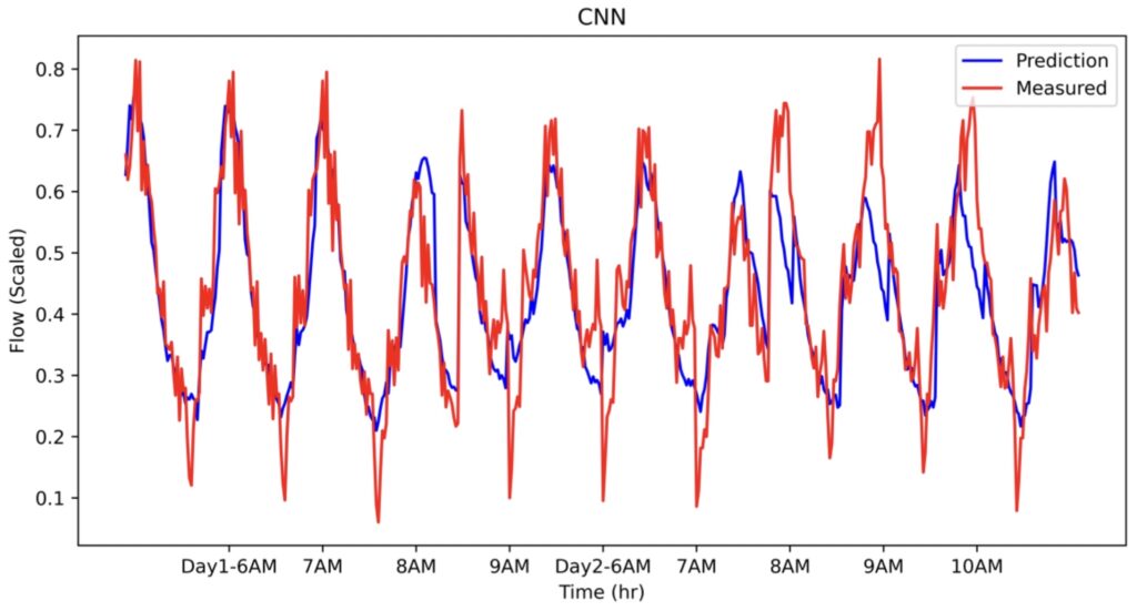
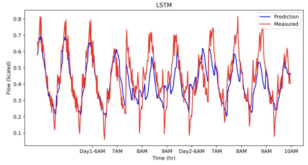
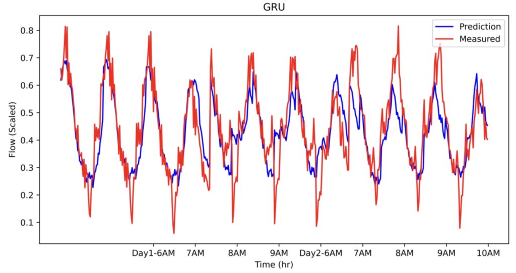
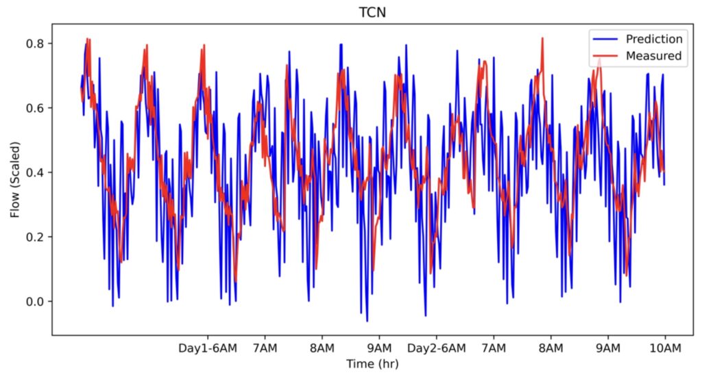
Figure 1. The comparison of measured traffic at E4S for two consecutive days between 6 to 10 AM obtained from a) CNN, b) LSTM, c) GRU, and d) TCN.
[1] P. Lara-Benitez, M. Carranza-Garcia, and J. C. Riquelme, Int. J. Neural Net., 31, 2130001 (2021).
[2] S. Bai, J. Z. Kolter, and V. Koltun, https://arxiv.org/abs/1803.01271 (2018).
[3] Y. He, and J. Zhao, J. Phys.: Conf. Ser. 1213, 042050 (2019).